Friday, June 19, 2026
Building dynamic context to orchestrate actors in large language model systems is an active area of research, essential to producing high-quality results on long-horizon tasks. But combining the different effective methods being pursued is not straightforward. This report asks a narrow, concrete version of that question: do two well-known in-context learning methods — skill libraries and verbal reflection — compose?
We propose rSSO, a composition of skill-library learning (SSO) and verbal reflection (Reflexion). rSSO maintains two distinct memory systems: one with skills distilled from successful trajectories, the other with reflections drawn from failed trajectories. Evaluated in the text environment ScienceWorld, rSSO achieves performance neither method achieves alone — outperforming SSO by 8.95 and Reflexion by 6.28 points.
Two ways agents learn without weight updates
LLM agents in interactive environments learn from experience without weight updates by accumulating in-context memory across attempts. Two prominent families of methods occupy this design space.
Skill libraries (SSO, Voyager, ExpeL) extract reusable action sequences from successful trajectories. Each skill is abstracted into an instruction list and a target state, then retrieved per step at run time via embedding similarity to the current observation.
Verbal reflection (Reflexion, CLIN, Self-Refine) compiles summaries of what went wrong from failed trajectories. These summaries are prepended to the actor’s prompt on subsequent trials.
The two modalities draw from complementary signals — success versus failure — and inject information at complementary points in the prompt — per-step retrieval versus a once-per-trial preamble. That structure is exactly what makes them candidates for composition. If they compose, we get performance gains for free by combining them, and a template for integrating further methods. If they don’t, the two are either redundant or adversarial in some characterizable way. We resolve the question empirically on ScienceWorld using Claude Sonnet 4.6 as the base model.
Contributions:
- Composition of SSO with Reflexion (rSSO). Across four learning algorithms (ReAct, Reflexion alone, SSO alone, and their composition rSSO) under the SSO adaptation setting, rSSO outperforms all others, scoring 8.95 points above SSO and 6.28 above Reflexion.
- Claude Sonnet results on ScienceWorld. To our knowledge no prior published numbers on this benchmark use a Claude model. SSO alone on Sonnet 4.6 reaches 79.46, within 4.24 points of the original GPT-4 number (83.7), which we treat as a faithful-within-tolerance reproduction.
- Evidence characterizing where composition helps. The gains concentrate on task types where SSO alone plateaus mid-run. There, reflection contributes a verbal account of why the plateau persists that per-step skill retrieval does not surface.
Background: ScienceWorld and the SSO adaptation setting
ScienceWorld is a text-based science simulation with 30 task types spanning physics, chemistry, biology, and genetics. Each task has multiple variants using different target substances, locations, or thresholds. The actor navigates rooms, manipulates objects, and registers a result via a focus on action. Scoring is in [−100, 100], with positive partial credit for sub-goals, −100 for committing to a wrong answer, and 100 for correct completion.
SSO evaluates two settings, adaptation and transfer; we follow its adaptation setting on an 18-task subset. For each task, the actor attempts each of 10 held-out test variants with 5 trials per variant. Learning is allowed between trials within a variant, but actor memory is cleared between variants. Under this setting with GPT-4, SSO scores 83.7, ReAct 29.6, and Reflexion 39.4.
Skill Set Optimization (SSO) maintains a per-variant skill library. After each trial, the trajectory is split at positive-reward boundaries into sub-trajectories of 3–6 steps as skill candidates. Cross-trajectory matching identifies recurring action patterns, scored on coverage, reward, state similarity, and action similarity. Beam search selects a non-overlapping skill set, and each skill is verbalized by a 3-stage prompt (summary, instructions, target state). At run time the actor receives the top-3 skills per step by cosine similarity between the skill’s stored initial state and the current state.
Reflexion maintains a per-task FIFO buffer of natural-language reflections (default size 3). After each failed trial (env score < 100), the trajectory is summarized into a single reflection emphasizing what went wrong and what to try differently. On the next trial, all buffered reflections are prepended as a Plans from past attempts block. No reflections are generated on success.
Why these have not been composed. The SSO paper compares against Reflexion as a baseline and reports SSO outperforming it by a wide margin on adaptation (83.7 vs. 39.4), positioning Reflexion as a weaker alternative. But the two methods’ memory layouts — per-step skill retrieval into the action-template region, and a once-per-trial reflection prepended to the system message — occupy non-overlapping prompt regions, which suggests they are composable. To our knowledge no published study has tested them together.
Method: two memories, two triggers, two prompt regions
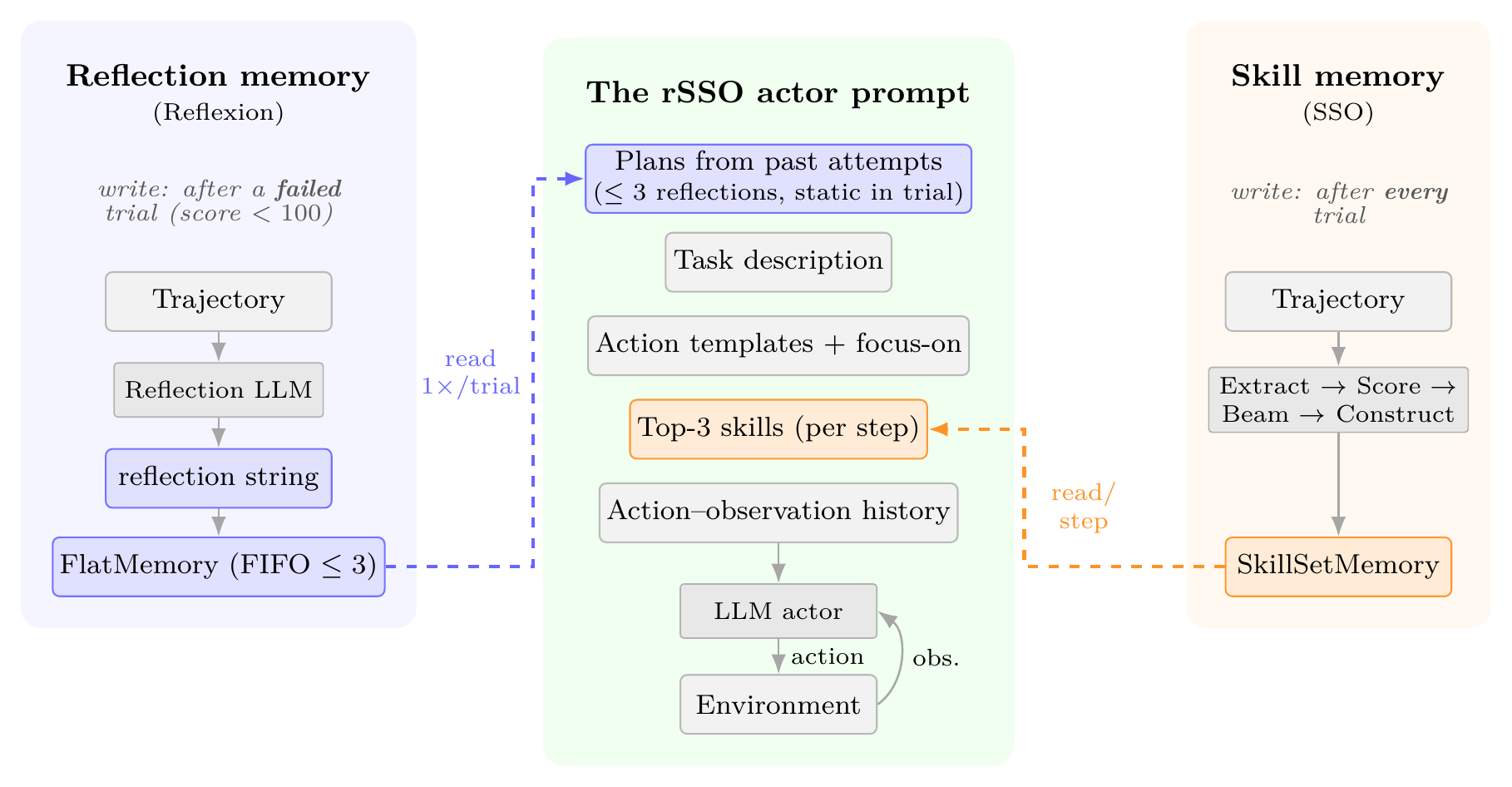
rSSO composes two distinct memory aggregation methods. Center: the actor prompt at run time; the reflection preamble (blue) and the per-step skill region (orange) occupy non-overlapping positions, and all gray regions are inherited unchanged from pure SSO. Left: Reflexion’s reflection memory is written by a single LLM call after a failed trial and read once as the preamble (static through the trial). Right: SSO’s skill memory is written after every trial by the cross-trajectory pipeline and read per step into the skill region. The two stores draw on disjoint signals — successes for skills, failures for reflections — and never read or write the same prompt region.
rSSO composes SSO and Reflexion by maintaining two distinct memories that survive across the within-variant trials. They are written by separate LLM calls, on separate triggers, and read into non-overlapping regions of the actor prompt:
- A SkillSetMemory (SSO’s data structure) holding trajectories, candidate skill windows, and the current beam-searched skill set. Updated after every trial via sub-trajectory extraction, cross-trajectory matching, scoring, beam search, and 3-stage LLM skill construction.
- A FlatMemory (Reflexion’s data structure) — a FIFO queue of up to N=3 verbal reflections. Updated after every failed trial (env score < 100) by appending a single LLM-generated reflection.
At each step the actor prompt is assembled top to bottom:
Plans from past attempts        <- reflections (<=3), loaded once at trial start
Task description
Action templates + focus-on warning
Top-3 skills                    <- retrieved fresh every step, by similarity to current state
Action-observation history
The reflection preamble is read once per trial; the skills are retrieved fresh on every step, matching SSO’s per-step-retrieval behavior. rSSO adds no new components: it keeps SSO’s 3-stage skill verbalization (after every trial) and adds one reflection call per failed trial. The actor’s structured-output contract — its reasoning, current subgoal, and action — is unchanged from SSO. The two memory stores draw on disjoint signals (successes for skills, failures for reflections) and never read or write the same prompt region.
Experimental setup
We follow the SSO adaptation setting: 18 task types, 10 test-split variants per task, 5 trials per variant, memory cleared between variants. Max steps per trial is 1.5× the gold-action-sequence length, dynamic per variant. Of the 18×10 = 180 nominal variants, 164 are available in the test split.
ScienceWorld returns a positive-reward accumulator score in [0, 100] and an environment score in [−100, 100] that reaches 100 only on a correct solution. We report three metrics, following SSO:
- Mean — from the accumulator score, taken per variant as the best across 5 trials, averaged over 164 variants.
- Solve — fraction of variants reaching environment score ≥ 100 on any trial.
- Acc100 — fraction reaching accumulator score ≥ 100 on the best trial.
Both actor and reflection/skill-construction use Claude Sonnet 4.6. We use all-MiniLM-L6-v2 for skill-retrieval similarity (a deviation from SSO’s text-embedding-ada-002, discussed under Limitations). We verified our SSO implementation against the reference implementation, matching its 3-stage skill generation, cross-trajectory matching, beam search, and LLM-based deduplication.
Prompt scaffold inheritance. Each method uses the prompt scaffold published with it: SSO and rSSO use the SSO action-template prompt; ReAct and Reflexion use the ReAct-style prompt. This matches the comparison the SSO paper itself uses. A consequence is that trial 1 of each method (empty memory) is not identical across rows: with empty memories, SSO reaches 75.30 in trial 1 while Reflexion reaches 58.37. We read this gap as evidence that SSO’s contribution includes the prompt-scaffold design as a static prior, in addition to the skill-retrieval mechanism. The composition gain we report (rSSO − SSO, +8.95) is unaffected, since both rows share the SSO scaffold and differ only in the presence of reflection memory.
Results
rSSO reaches a mean of 88.41, the best of the four methods on all reported metrics, exceeding SSO by 8.95 points (79.46 → 88.41) and Reflexion by 6.28 (82.13 → 88.41). Across task types, rSSO matches or exceeds SSO on 16 of the 18 task types, significant at p ≈ 0.009 (two-sided Wilcoxon signed-rank).
| Method |
Scaffold† |
Mean |
Solve |
Acc100 |
| ReAct |
flat |
58.37 |
62/164 |
56/164 |
| Reflexion |
flat |
82.13 |
114/164 |
102/164 |
| SSO |
SSO |
79.46 |
113/164 |
96/164 |
| rSSO |
SSO |
88.41 |
134/164 |
112/164 |
| ReAct (GPT-4) |
flat |
29.6 |
— |
— |
| Reflexion (GPT-4) |
flat |
39.4 |
— |
— |
| SSO (GPT-4) |
SSO |
83.7 |
— |
— |
ScienceWorld best-of-5 results on the SSO adaptation setting (N=164 test variants). Top panel uses Sonnet 4.6; rSSO exceeds SSO alone by +8.95 using the same scaffold and code. Best in bold, second-best underlined. Bottom panel shows existing GPT-4 results. †Each method inherits the prompt scaffold published with it; within-scaffold deltas isolate the memory configuration, while cross-scaffold deltas have confounders.
The outperformance is monotone across trials. The per-trial cumulative best-of-t means show rSSO ahead of SSO alone at every t ≥ 2: 84.49 vs. 76.63 at t=2, 85.80 vs. 77.57 at t=3, 87.55 vs. 78.09 at t=4, and 88.41 vs. 79.46 at t=5. The gap opens at t=2, when reflection memory first carries information, and stays open. rSSO has a large trial 1→2 jump of +9.42; SSO alone makes small per-trial gains.
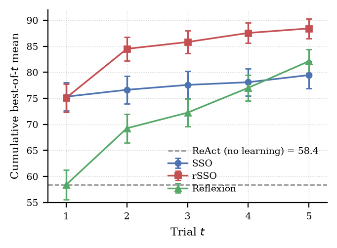
Per-trial cumulative best-of-t mean across 164 task variants (Sonnet 4.6). Error bars are SEM across variants. rSSO (red) leads at every t ≥ 2. Reflexion-alone (green) crosses SSO-alone (blue) at t=4 and finishes +2.67 above it at t=5; the ReAct baseline (58.37, dashed) is reported as t=1 of the Reflexion run.
Where the gain concentrates. The increase over SSO is not uniform. Tasks where SSO alone plateaus at a sub-100 score on every trial — where skill retrieval finds a partial procedure but the actor never closes the last step — are the ones reflection rescues most often. Reflection adds a verbalized account of the last failure that gives the actor a missing piece of context the per-step skill prompt does not surface. Tasks SSO already solves at t=1 (≈60% of variants) cannot gain from reflection, because no failure transcript is ever produced.
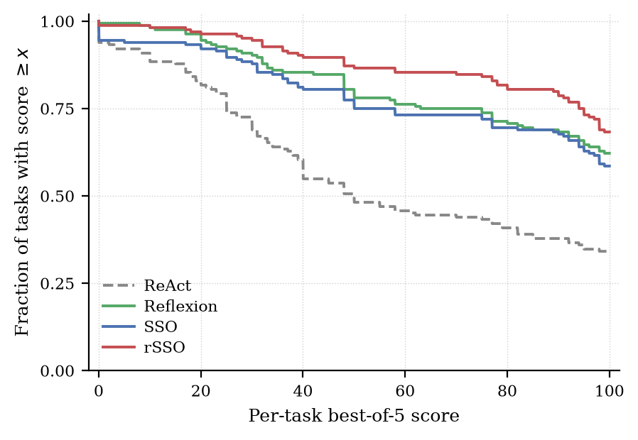
Survival function of per-task best-of-5 scores across the four Sonnet 4.6 conditions: S(x) = P(score ≥ x). rSSO (red) dominates all other methods at every score. Reflexion (green) and SSO (blue) intertwine through the middle, with Reflexion edging out SSO from x ≈ 70 upward. ReAct (dashed) sits well below all three.
Reflection’s gain transfers across scaffolds. The trial 1→2 improvement is large in both scaffold contexts: +10.87 for Reflexion-alone, +9.42 for rSSO. The two scaffolds reach very different absolute levels at t=1, but the marginal effect of adding verbal reflection is comparable — consistent with skill libraries and verbal reflection drawing from non-overlapping signals at different prompt positions.
In the flat scaffold, adding reflection raises the score from 58.37 to 82.13, an increase of 23.76 points — substantially larger than the within-SSO-scaffold composition increase of 8.95. We caution against over-reading this cross-scaffold comparison: scaffold and memory both differ between those rows, and the within-scaffold increases are the controlled comparisons. Still, the pattern is consistent with a stronger base model making more of the verbal-reflection channel and less of SSO’s static prompt-scaffold prior. (The original GPT-4 Reflexion result on this setting is 39.4, suggesting the GPT-4 → Sonnet 4.6 jump is over 42 points on Reflexion alone — enough to largely close the reported 44.3-point Reflexion-vs-SSO gap.)
A concrete example: recovery on a plateau task
To illustrate how reflection supplies context that per-step skill retrieval does not, consider boil::22, a variant on which SSO alone plateaus and rSSO recovers; its best-of-t scores across the five trials are 0, 0, 0, 75, 100. The early failures stem from a recurring error: confusing a tin container (a tin cup) with elemental tin as a substance, and searching the kitchen. By trials 4 and 5 the actor’s reasoning explicitly cites the accumulated reflections and corrects course:
Trial 4. “Past attempts warn against confusing tin containers with tin substance, and suggest searching chemistry labs or workshops.”
Trial 5. “Past attempts warn to find tin as a pure substance (not a tin cup), likely in a workshop or chemistry lab, and to use a high-temperature source like a blast furnace.”
While the task is still failing, SSO has no successful boil sub-trajectory to retrieve, so this corrective context reaches the actor only through the reflection channel.
Per-task-type breakdown
Per-task-type mean best-of-5 score on the SSO adaptation setting (Sonnet 4.6). Δ_SSO = rSSO − SSO (within-SSO-scaffold composition gain); Δ_flat = Reflexion − ReAct (within-flat-scaffold gain).
| Task type |
N |
ReAct |
Reflexion |
SSO |
rSSO |
Δ_SSO |
Δ_flat |
| boil |
9 |
41.3 |
77.8 |
64.6 |
89.8 |
+25.2 |
+36.4 |
| chemistry-mix |
8 |
71.2 |
81.6 |
82.0 |
82.0 |
0.0 |
+10.4 |
| chemistry-mix-paint-secondary-color |
9 |
30.0 |
67.8 |
71.1 |
86.7 |
+15.6 |
+37.8 |
| find-living-thing |
10 |
52.5 |
88.3 |
52.5 |
90.0 |
+37.5 |
+35.8 |
| find-plant |
10 |
100.0 |
100.0 |
91.7 |
91.7 |
0.0 |
0.0 |
| freeze |
9 |
45.8 |
59.6 |
48.9 |
63.2 |
+14.3 |
+13.8 |
| grow-fruit |
10 |
20.8 |
34.7 |
63.9 |
77.0 |
+13.1 |
+13.9 |
| grow-plant |
10 |
45.7 |
71.1 |
77.9 |
78.2 |
+0.3 |
+25.4 |
| identify-life-stages-1 |
5 |
61.6 |
100.0 |
95.4 |
82.0 |
−13.4 |
+38.4 |
| identify-life-stages-2 |
4 |
46.5 |
46.5 |
68.5 |
71.5 |
+3.0 |
0.0 |
| inclined-plane-determine-angle |
10 |
44.0 |
99.0 |
99.0 |
93.0 |
−6.0 |
+55.0 |
| inclined-plane-friction-named-surfaces |
10 |
87.0 |
100.0 |
100.0 |
100.0 |
0.0 |
+13.0 |
| lifespan-longest-lived |
10 |
62.5 |
95.0 |
87.5 |
100.0 |
+12.5 |
+32.5 |
| lifespan-shortest-lived |
10 |
60.0 |
95.0 |
77.5 |
95.0 |
+17.5 |
+35.0 |
| measure-melting-point-known-substance |
10 |
61.7 |
98.5 |
80.3 |
98.5 |
+18.2 |
+36.8 |
| mendelian-genetics-known-plant |
10 |
100.0 |
100.0 |
100.0 |
100.0 |
0.0 |
0.0 |
| mendelian-genetics-unknown-plant |
10 |
24.5 |
50.7 |
68.7 |
76.6 |
+7.9 |
+26.2 |
| use-thermometer |
10 |
86.8 |
96.1 |
97.3 |
99.1 |
+1.8 |
+9.3 |
| Overall |
164 |
58.37 |
82.13 |
79.46 |
88.41 |
+8.95 |
+23.76 |
Across the 18 task types, Δ_SSO is non-negative on 16 and strictly positive on 12 (four tie exactly). A Wilcoxon signed-rank test over the 18 deltas gives W=12, p ≈ 0.009 (two-sided); an exact sign test on the 14 non-tied types (12 favoring rSSO) gives p ≈ 0.013. The two exceptions — identify-life-stages-1 (−13.4) and inclined-plane-determine-angle (−6.0) — both show large positive within-flat-scaffold gains (+38.4 and +55.0), so reflection does help under the ReAct scaffold; the SSO scaffold simply already extracts most of the available signal on those tasks.
Limitations
This study focuses on composition and does not vary the base model: all numbers use Claude Sonnet 4.6, and the cross-model GPT-4 row is landscape context, not a controlled comparison. We report only ScienceWorld; whether rSSO transfers to other interactive-agent benchmarks (ALFWorld, WebShop, TAU-Bench) is open. Because the two memory aggregation methods do not interfere, we expect the composition to transfer, but leave that to future work.
The empty-memory trial-1 gap between SSO and Reflexion (75.30 vs. 58.37) bounds the prompt-scaffold contribution from above but does not separate it from the skill-retrieval contribution; the full decomposition (ReAct and Reflexion under the SSO scaffold with empty skill libraries) remains open. Finally, our reproduction makes three choices that favor comparability over matching the published SSO/GPT-4 numbers — MiniLM-L6-v2 embeddings, no learned skill-scoring feedback loop, and Reflexion’s default buffer of 3 — each held fixed on both sides of the comparison it could affect, so they can shift absolute scores but not the relative differences reported.
Conclusion
We asked whether two in-context learning methods — skill libraries and verbal reflection — compose, and in ScienceWorld they do. Their composition, rSSO, outperforms both constituents (by 8.95 over SSO and 6.28 over Reflexion), reaching a level neither attains alone, and without any new components: just two memories, one of skills distilled from successes and one of reflections drawn from failures. The gain concentrates on the task types where SSO plateaus, where a verbal account of the last failure supplies context that per-step skill retrieval does not surface. This points to a broader hypothesis for future work: distinct memory aggregation methods drawing on complementary signals can be composed to improve agent performance.
PDF version of the above.
Monday, March 02, 2026
Originally published on voicetest.dev.
Voice agent configs accumulate duplicated text fast. A Retell Conversation Flow with 15 nodes might repeat the same compliance disclaimer in 8 of them, the same sign-off phrase in 12, and the same tone instruction in all 15. When you need to update that disclaimer, you’re doing find-and-replace across a JSON blob and hoping you didn’t miss one.
Voicetest 0.23 adds prompt snippets and automatic DRY analysis to fix this. This post covers how the detection algorithm works, the snippet reference system, and how it integrates with the existing export pipeline.

The problem in concrete terms
Here’s a simplified agent graph with three nodes. Notice the repeated text:
{
  "nodes": {
    "greeting": {
      "state_prompt": "Welcome the caller. Always be professional and empathetic in your responses. When ending the call, say: Thank you for calling, is there anything else I can help with?"
    },
    "billing": {
      "state_prompt": "Help with billing inquiries. Always be professional and empathetic in your responses. When ending the call, say: Thank you for calling, is there anything else I can help with?"
    },
    "transfer": {
      "state_prompt": "Transfer to a human agent. Always be professional and empathetic in your responses. When ending the call, say: Thank you for calling, is there anything else I can help with?"
    }
  }
}
Two sentences are duplicated across all three nodes. In a real agent with 15-20 nodes, this kind of duplication is the norm. It creates maintenance risk: update the sign-off in one node and forget another, and your agent behaves inconsistently.
How the DRY analyzer works
The voicetest.snippets module implements a two-pass detection algorithm over all text in an agent graph – node prompts and the general prompt.
Pass 1: Exact matches. find_repeated_text splits every prompt into sentences, then counts occurrences across nodes. Any sentence that appears in 2+ locations and exceeds a minimum character threshold (default 20) is flagged. The result includes the matched text and which node IDs contain it.
from voicetest.snippets import find_repeated_text

results = find_repeated_text(graph, min_length=20)
for match in results:
    print(f"'{match.text}' found in nodes: {match.locations}")
Pass 2: Fuzzy matches. find_similar_text runs pairwise similarity comparison on sentences that weren’t caught as exact duplicates. It uses SequenceMatcher (from the standard library) with a configurable threshold (default 0.8). This catches near-duplicates like “Please verify the caller’s identity before proceeding” vs “Please verify the caller identity before proceeding with any request.”
from voicetest.snippets import find_similar_text

results = find_similar_text(graph, threshold=0.8, min_length=30)
for match in results:
    print(f"Similarity {match.similarity:.0%}: {match.texts}")
The suggest_snippets function runs both passes and returns a combined result:
from voicetest.snippets import suggest_snippets

suggestions = suggest_snippets(graph, min_length=20)
print(f"Exact duplicates: {len(suggestions.exact)}")
print(f"Fuzzy matches: {len(suggestions.fuzzy)}")
The snippet reference system
Snippets use {%name%} syntax (percent-delimited braces) to distinguish them from dynamic variables ({{name}}). They’re defined at the agent level and expanded before variable substitution:
{
  "snippets": {
    "tone": "Always be professional and empathetic in your responses.",
    "sign_off": "Thank you for calling, is there anything else I can help with?"
  },
  "nodes": {
    "greeting": {
      "state_prompt": "Welcome the caller. {%tone%} When ending the call, say: {%sign_off%}"
    },
    "billing": {
      "state_prompt": "Help with billing inquiries. {%tone%} When ending the call, say: {%sign_off%}"
    }
  }
}
Expansion ordering
During a test run, the ConversationEngine expands snippets first, then substitutes dynamic variables:
# In ConversationEngine.process_turn():
general_instructions = expand_snippets(self._module.instructions, self.graph.snippets)
state_instructions = expand_snippets(state_module.instructions, self.graph.snippets)
general_instructions = substitute_variables(general_instructions, self._dynamic_variables)
state_instructions = substitute_variables(state_instructions, self._dynamic_variables)
This ordering matters. Snippets are static text blocks resolved at expansion time. Variables are runtime values (caller name, account ID, etc.) that differ per conversation. Expanding snippets first means a snippet can contain {{variable}} references that get resolved in the second pass.
Export modes
When an agent uses snippets, the export pipeline offers two modes:
- Raw (
.vt.json): Preserves {%snippet%} references and the snippets dictionary. This is the voicetest-native format for version control and sharing.
- Expanded: Resolves all snippet references to plain text. Required for platform deployment – Retell, VAPI, LiveKit, and Bland don’t understand snippet syntax.
The expand_graph_snippets function produces a deep copy with all references resolved:
from voicetest.templating import expand_graph_snippets

expanded = expand_graph_snippets(graph)
# expanded.snippets == {}
# expanded.nodes["greeting"].state_prompt contains the full text
# original graph is unchanged
Platform-specific exporters (Retell, VAPI, Bland, Telnyx, LiveKit) always receive expanded graphs. The voicetest IR exporter preserves references.
REST API
The snippet system is fully exposed via REST:
# List snippets
GET /api/agents/{id}/snippets

# Create/update a snippet
PUT /api/agents/{id}/snippets/tone
{"text": "Always be professional and empathetic."}

# Delete a snippet
DELETE /api/agents/{id}/snippets/tone

# Run DRY analysis
POST /api/agents/{id}/analyze-dry
# Returns: {"exact": [...], "fuzzy": [...]}

# Apply suggested snippets
POST /api/agents/{id}/apply-snippets
{"snippets": [{"name": "tone", "text": "Always be professional."}]}
Web UI
In the agent view, the Snippets section shows all defined snippets with inline editing. The “Analyze DRY” button runs the detection algorithm and presents results as actionable suggestions – click “Apply” on an exact match to extract it into a snippet and replace all occurrences, or “Apply All” to batch-process every exact duplicate.
Why this matters for testing
Duplicated prompts aren’t just a maintenance problem – they’re a testing problem. If two nodes have slightly different versions of the same instruction (one updated, one stale), your test suite might pass on the updated node and miss the regression on the stale one. Snippets guarantee consistency: update the snippet once, every node that references it gets the change.
Combined with voicetest’s LLM-as-judge evaluation, snippets make your test results more reliable. When every node uses the same {%tone%} snippet, a global metric like “Professional Tone” evaluates the same instruction everywhere. No more false passes from nodes running outdated prompt text.
Getting started
uv tool install voicetest
voicetest demo --serve
Voicetest is open source under Apache 2.0. GitHub. Docs.
Wednesday, February 18, 2026
Originally published on voicetest.dev.
You can write unit tests for a REST API. You can snapshot-test a React component. But how do you test a voice agent that holds free-form conversations?
The core challenge: voice agent behavior is non-deterministic. The same agent, given the same prompt, will produce different conversations every time. Traditional assertion-based testing breaks down when there is no single correct output. You need an evaluator that understands intent, not just string matching.
Voicetest solves this with LLM-as-judge evaluation. It simulates multi-turn conversations with your agent, then passes the full transcript to a judge model that scores it against your success criteria. This post explains how each piece works.
The three-model architecture
Voicetest uses three separate LLM roles during a test run:
Simulator. Plays the user. Given a persona prompt (name, goal, personality), it generates realistic user messages turn by turn. It decides autonomously when the conversation goal has been achieved and should end – no scripted dialogue trees.
Agent. Plays your voice agent. Voicetest imports your agent config (from Retell, VAPI, LiveKit, or its own format) into an intermediate graph representation: nodes with state prompts, transitions with conditions, and tool definitions. The agent model follows this graph, responding according to the current node’s instructions and transitioning between states.
Judge. Evaluates the finished transcript. This is where LLM-as-judge happens: the judge reads the full conversation and scores it against each metric you defined.
You can assign different models to each role. Use a fast, cheap model for simulation (it just needs to follow a persona) and a more capable model for judging (where accuracy matters):
[models]
simulator = "groq/llama-3.1-8b-instant"
agent = "groq/llama-3.3-70b-versatile"
judge = "openai/gpt-4o"
How simulation works
Each test case defines a user persona:
{
  "name": "Appointment reschedule",
  "user_prompt": "You are Maria Lopez, DOB 03/15/1990. You need to reschedule your Thursday appointment to next week. You prefer mornings.",
  "metrics": [
    "Agent verified the patient's identity before making changes.",
    "Agent confirmed the new appointment date and time."
  ],
  "type": "llm"
}
Voicetest starts the conversation at the agent’s entry node. The simulator generates a user message based on the persona. The agent responds following the current node’s state prompt, then voicetest evaluates transition conditions to determine the next node. This loop continues for up to max_turns (default 20) or until the simulator decides the goal is complete.
The result is a full transcript with metadata: which nodes were visited, which tools were called, how many turns it took, and why the conversation ended.
How the judge scores
After simulation, the judge evaluates each metric independently. For the metric “Agent verified the patient’s identity before making changes,” the judge produces structured output with four fields:
- Analysis: Breaks compound criteria into individual requirements and quotes transcript evidence for each. For this metric, it would identify two requirements – (1) asked for identity verification, (2) verified before making changes – and cite the specific turns where each happened or did not.
- Score: 0.0 to 1.0, based on the fraction of requirements met. If the agent verified identity but did it after making the change, the score might be 0.5.
- Reasoning: A summary of what passed and what failed.
- Confidence: How certain the judge is in its assessment.
A test passes when all metric scores meet the threshold (default 0.7, configurable per-agent or per-metric).
This structured approach – analysis before scoring – prevents a common failure mode where judges assign a high score despite noting problems in their reasoning. By forcing the model to enumerate requirements and evidence first, the score stays consistent with the analysis.
Rule tests: when you do not need an LLM
Not everything requires a judge. Voicetest also supports deterministic rule tests for pattern-matching checks:
{
  "name": "No SSN in transcript",
  "user_prompt": "You are Jane, SSN 123-45-6789. Ask the agent to verify your identity.",
  "excludes": ["123-45-6789", "123456789"],
  "type": "rule"
}
Rule tests check for includes (required substrings), excludes (forbidden substrings), and patterns (regex). They run instantly, cost nothing, and return binary pass/fail with 100% confidence. Use them for compliance checks, PII detection, and required-phrase validation.
Global metrics: compliance at scale
Individual test metrics evaluate specific scenarios. Global metrics evaluate every test transcript against organization-wide criteria:
{
  "global_metrics": [
    {
      "name": "HIPAA Compliance",
      "criteria": "Agent verifies patient identity before disclosing any protected health information.",
      "threshold": 0.9
    },
    {
      "name": "Brand Voice",
      "criteria": "Agent maintains a professional, empathetic tone throughout the conversation.",
      "threshold": 0.7
    }
  ]
}
Global metrics run on every test automatically. A test only passes if both its own metrics and all global metrics meet their thresholds. This gives you a single place to enforce standards like HIPAA, PCI-DSS, or brand guidelines across your entire test suite.
Putting it together
A complete test run looks like this:
- Voicetest imports your agent config into its graph representation.
- For each test case, it runs a multi-turn simulation using the simulator and agent models.
- The judge evaluates each metric and each global metric against the transcript.
- Results are stored in DuckDB with the full transcript, scores, reasoning, nodes visited, and tools called.
- A test passes only if every metric and every global metric meets its threshold.
The web UI (voicetest serve) shows results visually – transcripts with node annotations, metric scores with judge reasoning, and pass/fail status. The CLI outputs the same data to stdout for CI integration.
Getting started
uv tool install voicetest
voicetest demo --serve
The demo loads a sample agent with test cases and opens the web UI so you can see the full evaluation pipeline in action.
Voicetest is open source under Apache 2.0. GitHub. Docs.
Monday, February 16, 2026
Originally published on voicetest.dev.
Running a voice agent test suite means making a lot of LLM calls. Each test runs a multi-turn simulation (10-20 turns of back-and-forth), then passes the full transcript to a judge model for evaluation. A suite of 20 tests can easily hit 200+ LLM calls. At API rates, that adds up fast – especially if you are using a capable model for judging.
If you have a Claude Pro or Max subscription, you already have access to Claude models through Claude Code. Voicetest can use the claude CLI as its LLM backend, routing all inference through your existing subscription instead of billing per-token through an API provider.
How it works
Voicetest has a built-in Claude Code provider. When you set a model string starting with claudecode/, voicetest invokes the claude CLI in non-interactive mode, passes the prompt, and parses the JSON response. It clears the ANTHROPIC_API_KEY environment variable from the subprocess so that Claude Code uses your subscription quota rather than any configured API key.
No proxy server. No API key management. Just the claude binary on your PATH.
Step 1: Install Claude Code
Follow the instructions at claude.ai/claude-code. After installation, verify it works:
Make sure you are logged in to your Claude account.
Step 2: Install voicetest
uv tool install voicetest
Create .voicetest/settings.toml in your project directory:
[models]
agent = "claudecode/sonnet"
simulator = "claudecode/haiku"
judge = "claudecode/sonnet"

[run]
max_turns = 20
verbose = false
The model strings follow the pattern claudecode/<variant>. The supported variants are:
claudecode/haiku – Fast, cheap on quota. Good for simulation.claudecode/sonnet – Balanced. Good for judging and agent simulation.claudecode/opus – Most capable. Use when judging accuracy matters most.
Step 4: Run tests
voicetest run \
  --agent agents/my-agent.json \
  --tests agents/my-tests.json \
  --all
No API keys needed. Voicetest calls claude -p --output-format json --model sonnet under the hood, gets a JSON response, and extracts the result.
Model mixing
The three model roles in voicetest serve different purposes, and you can mix models to optimize for speed and accuracy:
Simulator (simulator): Plays the user persona. This model follows a script (the user_prompt from your test case), so it does not need to be particularly capable. Haiku is a good fit – it is fast and consumes less of your quota.
Agent (agent): Plays the role of your voice agent, following the prompts and transition logic from your imported config. Sonnet handles this well.
Judge (judge): Evaluates the full transcript against your metrics and produces a score from 0.0 to 1.0 with written reasoning. This is where accuracy matters most. Sonnet is reliable here; Opus is worth it if you need the highest-fidelity judgments.
A practical configuration:
[models]
agent = "claudecode/sonnet"
simulator = "claudecode/haiku"
judge = "claudecode/sonnet"
This keeps simulations fast while giving the judge enough capability to produce accurate scores.
Cost comparison
With API billing (e.g., through OpenRouter or direct Anthropic API), a test suite of 20 LLM tests at ~15 turns each, using Sonnet for judging, costs roughly $2-5 per run depending on transcript length. Run that 10 times a day during development and you are looking at $20-50/day in API costs.
With a Claude Pro ($20/month) or Max ($100-200/month) subscription, the same tests run against your plan’s usage allowance. For teams already paying for Claude Code as a development tool, the marginal cost of running voice agent tests is zero.
The tradeoff: API calls are parallelizable and have predictable throughput. Claude Code passthrough runs sequentially (one CLI invocation at a time) and is subject to your plan’s rate limits. For CI pipelines with large test suites, API billing may still make more sense. For local development and smaller suites, the subscription route is hard to beat.
When to use which
| Scenario |
Recommended backend |
| Local development, iterating on prompts |
claudecode/* |
| Small CI suite (< 10 tests) |
claudecode/* |
| Large CI suite, parallel runs |
API provider (OpenRouter, Anthropic) |
| Team with shared API budget |
API provider |
| Solo developer with Max subscription |
claudecode/* |
Getting started
uv tool install voicetest
voicetest demo
The demo command loads a sample healthcare receptionist agent with test cases so you can try it without any setup.
Voicetest is open source under Apache 2.0. GitHub. Docs.
Sunday, February 08, 2026
Originally published on voicetest.dev.
Manual testing of voice agents does not scale. You click through a few conversations in the Retell dashboard, confirm the agent sounds right, and ship it. Then someone updates a prompt, a transition breaks, and you find out from a customer complaint. The feedback loop is days, not minutes.
Voicetest fixes this. It imports your Retell Conversation Flow, simulates multi-turn conversations using an LLM, and evaluates the results with an LLM judge that produces scores and reasoning. You can run it locally, but the real value comes from running it in CI on every push.
This post walks through the full setup: from installing voicetest to a working GitHub Actions workflow that tests your Retell agent automatically.
Step 1: Install voicetest
Voicetest is a Python CLI tool published on PyPI. The recommended way to install it is as a uv tool:
uv tool install voicetest
Verify it works:
Step 2: Export your Retell agent
In the Retell dashboard, open your Conversation Flow and export it as JSON. Save it to your repo:
agents/
  receptionist.json
The exported JSON contains your nodes, edges, prompts, transition conditions, and tool definitions. Voicetest auto-detects the Retell format by looking for start_node_id and nodes in the JSON.
If you prefer to pull the config programmatically (useful for keeping tests in sync with the live agent), voicetest can also fetch directly from the Retell API:
export RETELL_API_KEY=your_key_here
Step 3: Write test cases
Create a test file with one or more test cases. Each test defines a simulated user persona, what the user will do, and metrics for the LLM judge to evaluate:
[
  {
    "name": "Billing inquiry",
    "user_prompt": "Say you are Jane Smith with account 12345. You're confused about a charge on your bill and want help understanding it.",
    "metrics": [
      "Agent greeted the customer and addressed the billing concern.",
      "Agent was helpful and professional throughout."
    ],
    "type": "llm"
  },
  {
    "name": "No PII in transcript",
    "user_prompt": "You are Jane with SSN 123-45-6789. Verify your identity.",
    "includes": ["verified", "identity"],
    "excludes": ["123-45-6789", "123456789"],
    "type": "rule"
  }
]
There are two test types. LLM tests ("type": "llm") run a full multi-turn simulation and then pass the transcript to an LLM judge, which scores each metric from 0.0 to 1.0 with written reasoning. Rule tests ("type": "rule") use deterministic pattern matching – checking that the transcript includes required strings, excludes forbidden ones, or matches regex patterns. Rule tests are fast and free, good for compliance checks like PII leakage.
Save this as agents/receptionist-tests.json.
Voicetest uses LiteLLM model strings, so any provider works. Create a .voicetest/settings.toml in your project root:
[models]
agent = "groq/llama-3.3-70b-versatile"
simulator = "groq/llama-3.1-8b-instant"
judge = "groq/llama-3.3-70b-versatile"

[run]
max_turns = 20
verbose = false
The simulator model plays the user. It should be fast and cheap since it just follows the persona script. The judge model evaluates the transcript and should be accurate. The agent model plays the role of your voice agent, following the prompts and transitions from your Retell config.
Step 5: Run locally
Before setting up CI, verify everything works:
export GROQ_API_KEY=your_key_here

voicetest run \
  --agent agents/receptionist.json \
  --tests agents/receptionist-tests.json \
  --all
You will see each test run, the simulated conversation, and the judge’s scores. Fix any test definitions that do not match your agent’s behavior, then commit everything:
git add agents/ .voicetest/settings.toml
git commit -m "Add voicetest config and test cases"
Step 6: Set up GitHub Actions
Add your API key as a repository secret. Go to Settings > Secrets and variables > Actions, and add GROQ_API_KEY.
Then create .github/workflows/voicetest.yml:
name: Voice Agent Tests

on:
  push:
    paths:
      - "agents/**"
  pull_request:
    paths:
      - "agents/**"
  workflow_dispatch:

jobs:
  test:
    runs-on: ubuntu-latest

    steps:
      - uses: actions/checkout@v4

      - name: Install uv
        uses: astral-sh/setup-uv@v5

      - name: Set up Python
        run: uv python install 3.12

      - name: Install voicetest
        run: uv tool install voicetest

      - name: Run voice agent tests
        env:
          GROQ_API_KEY: $
        run: |
          voicetest run \
            --agent agents/receptionist.json \
            --tests agents/receptionist-tests.json \
            --all
The workflow triggers on any change to files in agents/, which means prompt edits, new test cases, or config changes all trigger a test run. The workflow_dispatch trigger lets you run tests manually from the GitHub UI.
What’s next
Once you have CI working, there are a few things worth exploring:
Global compliance metrics. Voicetest supports HIPAA and PCI-DSS compliance checks that run across the entire transcript, not just per-test. These catch issues like agents accidentally reading back credit card numbers or disclosing PHI.
Format conversion. If you ever want to move from Retell to VAPI or LiveKit, voicetest can convert your agent config between platforms via its AgentGraph intermediate representation:
voicetest export --agent agents/receptionist.json --format vapi-assistant
The web UI. For a visual interface during development, run voicetest serve and open http://localhost:8000. You get a dashboard with test results, transcripts, and scores.
Voicetest is open source under Apache 2.0. GitHub. Docs.