Covid 19 Time Series Analysis
Sunday, March 15, 2020COVID-19 Time Series Analysis
Here we analyze the COVID-19 case data to create simple charts and time series models. This is meant as a review of time series analysis methods and not to accurately predict the future course of the pandemic. These models are based on the daily case data only, they are all univariate, and they do not consider environmental changes (e.g. travel restrictions, quarantines, and event cancellations).
The rest of this post describes the functionality of the COVID-19 Time Series Analysis IPython Notebook and includes charts with the data available as of March 15th, 2020. Feel free to use, modify, extend, and contribute to the notebook.
Fetch COVID historical case date
Each time we run the build_data function we will:
- retrieve data from the Johns Hopkins Center for Systems Science and Engineering,
- merge data into a single Pandas DataFrame.
This fetches all data available in the CSSEGIS COVID-19 repository at the time it is run.
Reformat data for visualization and modeling
Use the unify_names function to combine multiple countries and/or provinces/states into a single country. This resolves problems when the names of single countries are inconsistent in the CSSEGIS datasets.
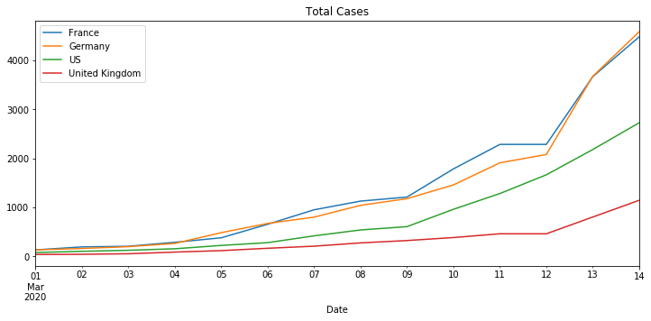
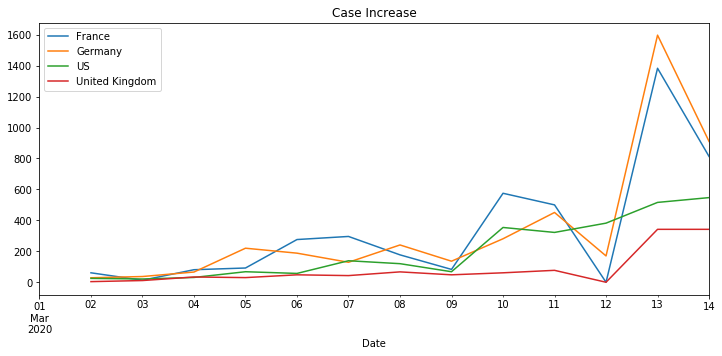
Use the plot function to produce total cases and case per day charts for a set of countries and metrics, passed as parameters.
Naive Time Series Models
This section requires that the grouped_df DataFrame and the all_countries list exist. These models are not run in parallel, but they can be. These models are incredibly naive, we are only considering the previous case numbers, nothing exogenous.
Use the prepare_data function to limit the countries and metrics. Currently this can model univariate data, i.e. it only considers a single country (or province/state) at a time. It would be interesting to use VAR or other multivariate models to capture the interdependence between countries.
We have written forecasting functions that use the ARIMA and Holt Winters Exponential Smoothing time series analysis methods. Additional forecasting methods in the same format as these functions should work fine.
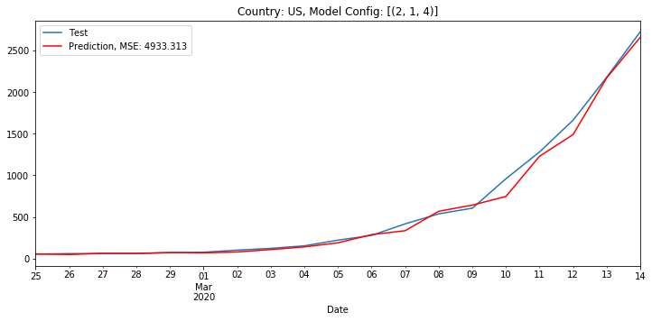
The grid_search function takes a map from forecasting functions to a list of configurations per forecasting function and evaluates all configurations using a walk forward method with a 2/3rds training and testing split. There is no validation or cross-validation step. This function returns a list of forecast function, configuration, and mean squared error (MSE) tuples ordered by increasing (i.e. worse) MSE.
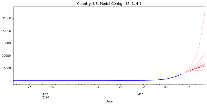
On March 15th, 2020, when evaluating the US case count, an ARIMA model with order (2, 1, 4) had the lowest MSE of 4,933. The below chart plots the actual and predicted values for the testing data.
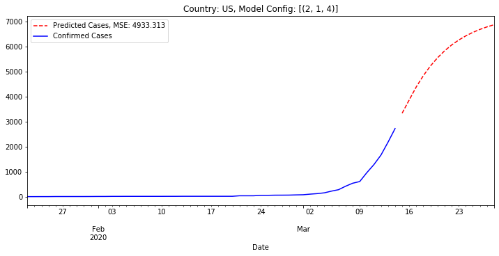
Below is the result if we have this best fit model (best as in lowest MSE) predict the number of cases for the next two weeks. The gap is because we do not connect the last day of actual data to the first day of predicted data. We show predicted cases as a red dotted line.
Looking at a wider set of models, below is the result for the next week showing all models with a MSE below 20,000 in pink and the best model in dark red. We see that when considering all our models there are a variety of possible outcomes.
There are many other factors and methods that would improve these models. This is meant as a review of time series analysis methods and not to accurately predict the future course of the pandemic. Please take a look at the COVID-19 Time Series Analysis IPython Notebook to explore and extend the code.